1. Framework
SoyOmics is a database providing comprehensive knowledge and analysis tools for soybean multi-omics. We de novo assembled 27 genomes of different soybean accessions, generated ~550 thousand large scale structural variations (SVs) and built graph pan-genome (Liu et al., 2020). We collected ~3,000 soybean germplasms and generated ~38 million SNPs and INDELs from them (Zhou et al., 2015; Fang et al., 2017; Liu et al., 2020). Besides, we generated 28 or 9 tissue-stages gene expression data of ZH13/WM82 or pan-genome accessions (Shen et al., 2014; Shen et al., 2019; Liu et al., 2020), and ~27 thousand records of 115 soybean phenotypes from different years and areas of planting. The multi-omics data can be classed into 6 basic modules: Genome, Variome, Transcriptome, Phenome, Homology and Synteny. After that, we provide analysis tools for BLAST search (BLAST), GWAS (easyGWAS), gene expression pattern (ExpPattern), haplotype (HapSnap), genome position transform (VersionMap) and Soybean array (SoyArray).
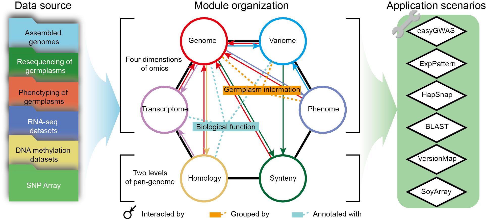
Figure 1 Framework of
SoyOmics
2. Search
The "Search" bar on homepage provides global search of all related items or directional search for input type.
- Region: an input form as "chromosome:start-end" is supported.
- Genes/Symbol: the complete/incomplete gene ID or symbol are legal input for search.
- Variation: the "chromosome:position" type or variation ID are both accepted.
- Accession: the accession ID, English or Chinese are all supported.
- Phenotype: the abbreviation and English/Chinese full title are accessible.
We support the high integration of the searching result. You can get a quick start in the "Search" function, from which one can be informed with all basic knowledge in the database and walk to the details.

Figure 2 Search
3.1. Accession list
The main page of Genome module embodies the information of 2,898 soybean germplasms, 27 of which contains de novo assembled genome. The distribution, phylogeny, accession information and de novo assembly statistics can be found here.

Figure 3.1 Accessions
3.2. Accession details
The accession's private page contains detailed information and genome view (if possible) for each accession. The gene number statistics, JBrowse, and synteny can be found here. Clicking on the gene number can redirect to the gene search panel.

Figure 3.2 Accession
details
3.3. Gene search panel
In SoyOmics, mRNA and other non-coding RNA were annotated for all de novo assembled genomes. One can use assembly name, gene type and/or genomic region to narrow the present gene list or use gene ID to directly lock on any interesting gene. All gene's private page can be visited from the list.

Figure 3.3 Gene search
3.4. Gene details
We designed exhibition framework for each single gene. This framework shows 9 parts such as basic summary, molecular functional annotation, biological knowledge, overlapped variation, homology, and gene expression pattern. You can fast locate to any part that you are interested in. From this detailed page, you can jump to the variations within the gene, homologous group or expression pattern from the gene's page.
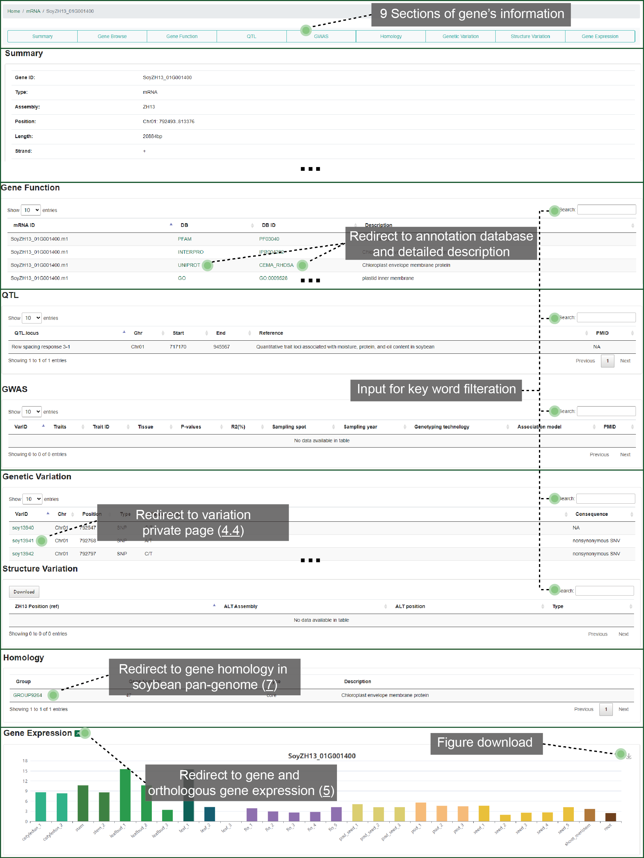
Figure 3.4 Gene
details
4. Variome module
The Variome module organizes the SNPs and INDELs of the 2,898 soybean accessions. The main page of Variome contains three parts: variation statistics, selective test and variation browser.
4.1. Variation Statistics
The variation statistics provides an overview of SNP and Indel density through the chromosomes and the annotation statistics summary.

Figure 4.1 Variation
statistics
4.2. Selective test
Three measures, Tajima’s D, FST and ROD, are used for whole genome selective test. Tracks and regions can be identified as you like. Threshold of the top 5% is drawn by a dash line. Figure of selective test can be downloaded.
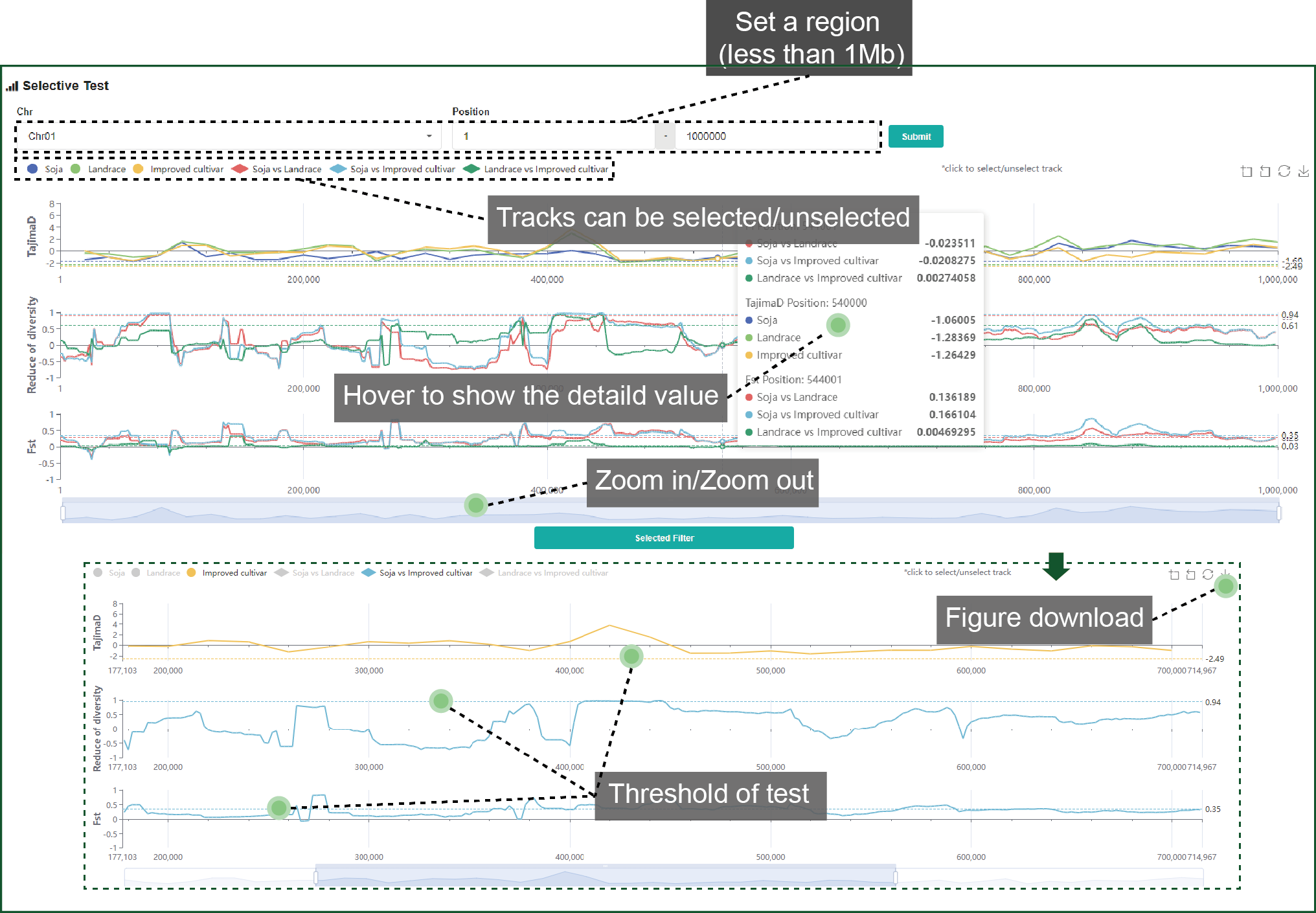
Figure 4.2 Selective
test
4.3. Variation Browser
In variation Browser, you can customize the conditions to restrict the variation list. We provide four items for filtration:
- "Position and Type" identifies the searching region, and the SNP and/or INDEL type;
- "Consequence Type" identifies how the variations change the protein;
- "Variation Annotation" rules whether the variations overlap with reported biological knowledge or linkage disequilibrium (LD) blocks;
- "Frequency" limits the minor allele frequency (MAF) and missing rate of variations.
Variation list can be downloaded with certain accessions. You can redirect to the variation's private page from here.
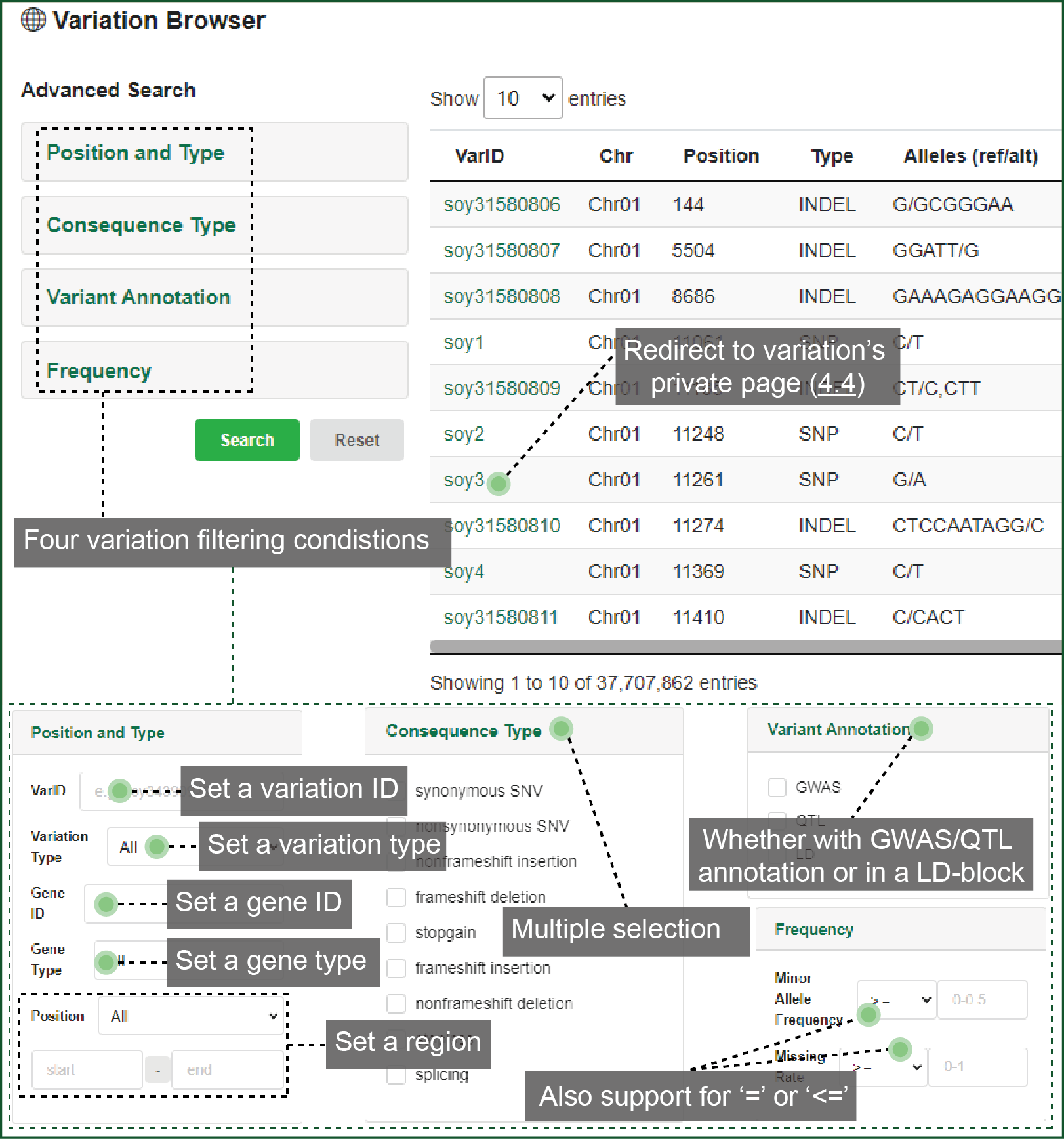
Figure 4.3 Variation
browse
4.4.1. Basic information
On the private page of single variation, 8 parts of information are displayed. You can fast locate to a certain part or redirect to the overlapped gene.

Figure 4.4.1 Variation
basic information
4.4.2. LD block
This part draws the LD block if the variation is involved in. The R2 can be set as threshold for drawing LD heat map and displaying variation in table. Other variations involved in the same LD block can be directly visited from here. The LD heat map can be downloaded.

Figure 4.4.2 LD block
4.4.3 Population statistics
This part concludes the population statistics of the variation. The allele, genotype and missing frequency are drawn as column charts. These column charts can be divided by population type (soja, landrance, and cultivar) or further drawn as percent stacked. When grouped by population type, the pie chart was drawn for each type with different allele or genotype ratio. All figures can be downloaded.
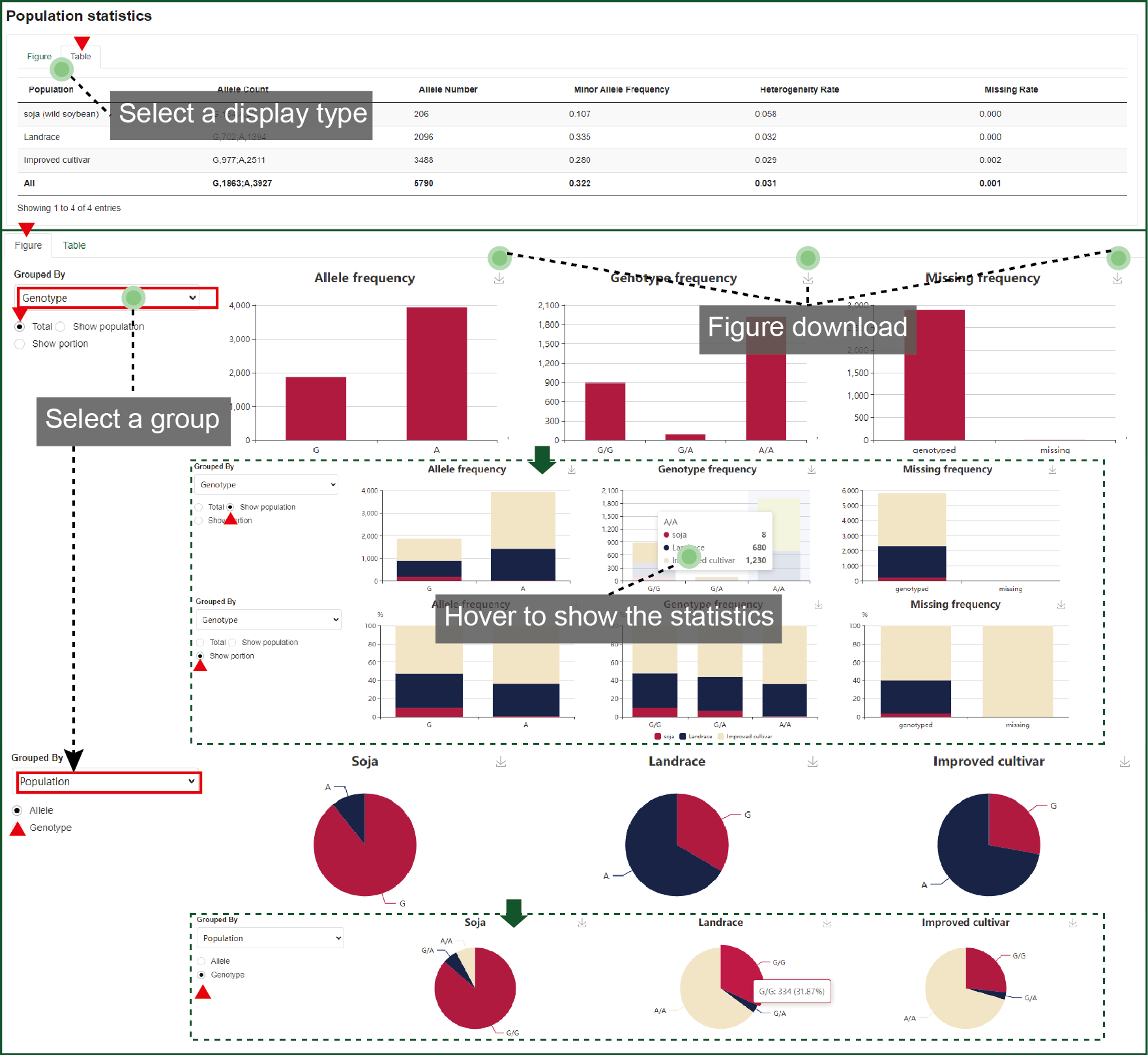
Figure 4.4.3
Population
statistics
4.4.4 Phenotype associated to variation
This part draws relationship between variation and phenotypes. Boxplot is generated by genotypes of this variation site against the value after best linear unbiased prediction (BLUP) of all the 115 phenotypes. Figures can be directly downloaded.

Figure 4.4.4 Phenotype
to
variation association
5. Transcriptome module
In the Transcriptome module, we afford two datasets of gene expression. One contain expression of 27 tissues from different developmental stages and organs for ZH13 and WM82 accession respectively. The other contain expression of 9 tissues from different developmental stages and organs for 26 accessions of pan-genome project. When searching a gene in this module, it returns the column chart of FPKM in the available tissues. If the gene has orthologous gene in the pan-genome, the heat map of orthologous genes' FPKM against 9 tissue-stages will also returned. Notice that you can also search the word related to gene function by the "Gene Function". The transcriptome module can redirect to the gene private page.
Figure 5 Transcriptome
6. Phenome module
In the Phenome module, 115 phenotypes are classed into a 3-levels catalogue. The phenotype records were achieved during 2013~2015 from Beijing, Henan, Heilongjiang, and Shanxi. You can quickly select a phenotype by interacting with the sunburst graph. Those phenotype records are firstly counted with different qualitative tags or quantitative value regions. Then the accessions with phenotypic value are grouped by sample types (soja, landrace, and cultivar), countries and eco-regions of China.

Figure 6 Phenome
7. Homology module
We load information of 57,479 homologous groups of the pan-genome, including genes of WM82 and W05, into this module. You can use gene ID, functional description or group name to search the homologous groups. Column chart show the number of genes in each genome. The gene list can be filtered, hidden or displayed. You can visit every gene's private page of a group, and achieve the alignment of CDS and protein sequences or phylogenic tree.

Figure 7 Homology
8. Synteny module
This module provides a function visualize the pan-genome by synteny blocks, SVs, and tubemap of graph genome.
8.1 Chromosome synteny
In this part, you can set the query strain, chromosome and region to see the dynamic synteny and SV distribution. The synteny and SV list can be synchronized with the inputting region and prepared for download.
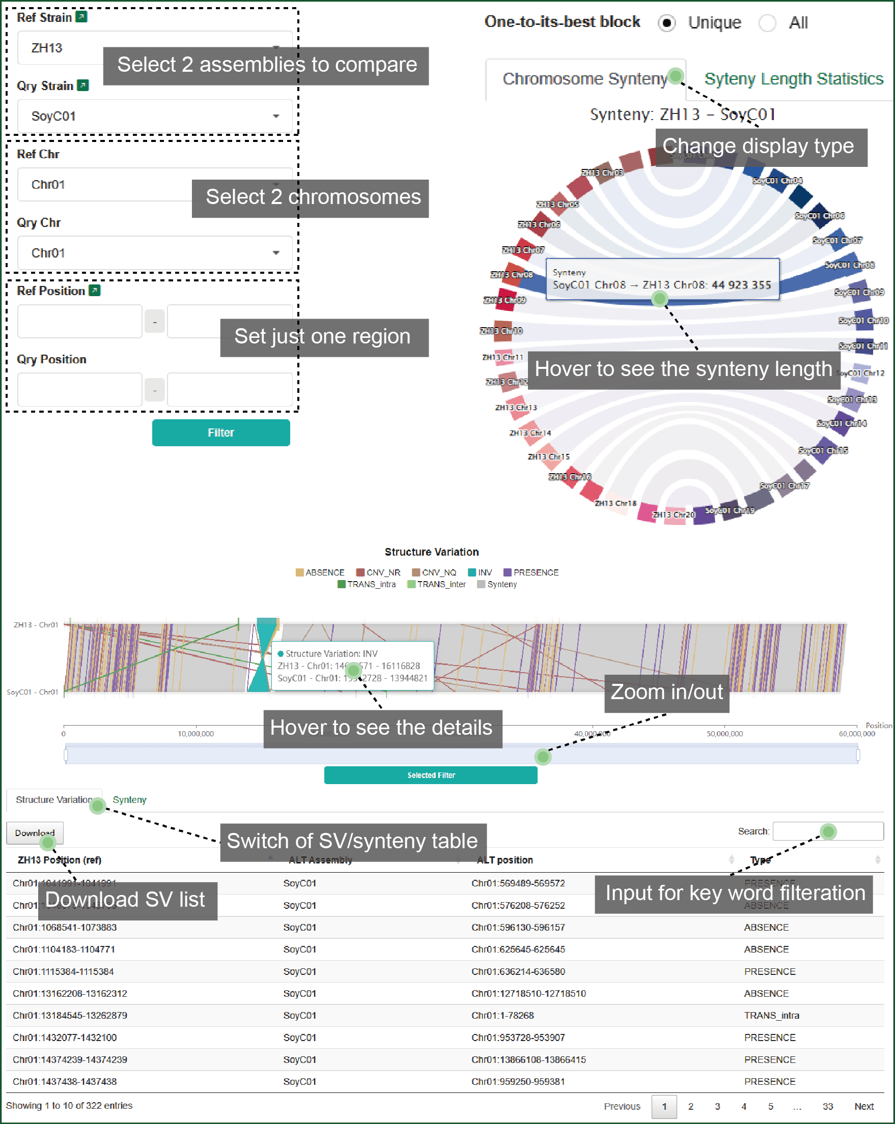
Figure 8 Synteny
8.2 Graph genome
In this part, you can set a genomic region of ZH13 to generated the haplotypes (threads) of de novo soybeans according to SVs and visualize the tubemap from graph genome. Key nodes for deciding the haplotypes will be shown in the table. Corresponding nodes can also be found on the tubemap.

9. JBrowse
Genome browser is launched by JBrowse. The ZH13 is provided as reference genome. The gene annotation, GC, domestication region, QTL, variation and other omics such as methylation , are also can be viewed.

Figure 9 Jbrowse
10. Online tools
10.1. easyGWAS
10.1.1. GWAS submission
easyGWAS provides three datasets as genotype, the SNP from WGS of 2,898 accessions, the SNP from GenoBaits Soy40K array, and genotype uploading by yourself. The MAF and missing rate filtration can be set as genotype quality control. EMMAX, GEMMA, or Plink can be chose for GWAS calculation. Other parameters such as PCA option and threshold setting are afforded. If you would like to upload genotype by yourself, the block-gzipped vcf file lower than 300 Mb is accepted.

Figure 10.1.1 GWAS
submission
10.1.2. GWAS result
After calculating, result will display the full parameters you have set, and show the Manhattan plot and QQ-plot of GWAS, with sites over the threshold highlighted. The complete GWAS results and figures can be downloaded.

Figure 10.1.2 GWAS
result
10.2. ExpPattern assists data mining
ExpPattern draws the gene-tissue expression heat map with cluster and estimate the tissue specific level. For query input, gene ID, gene symbol, annotation ID, and functional description of gene are all accepted. Other parameters including FPKM filtration threshold and log-normalization also can be chose. Any gene or tissue in the table can be selected/unselected on the table to remake the heat map, with options of whether to execute cluster. The tspex is embedded in the Transcri-pattern for advice of gene's tissue-specificity. The Tau and Simpson index are used for general scoring metrics, meanwhile the Tissue-specificiy index (TSI), Z-score and SPM are used for individualized scoring metrics. For more reasonable analysis of the gene expression and tissue-specificity, we provide the option of tissue group.

Figure 10.2
ExpPattern
10.3. HapSnap
HapSnap supports haplotype analysis with the SNP/INDEL data of the 2,898 soybeans and 115 phenotypes. Firstly, the target region can be identified as “chromosome:start-end”, or as the “gene ID” + “up/down-stream length”. Secondly, the variation types can be freely combined to make up the haplotypes. Thirdly, the missing rate, minor allele frequency and heterozygous rate can be set as the filtration criteria. After haplotypes are defined, the haplotype frequency, haplotype vs. genotype, linkage disequilibrium will be calculated.

Figure 10.3 HapSnap
10.4. BLAST
10.4.1. BLAST submission
The genome, CDS, protein sequences of 28 accessions are provided for BLAST. You can input at most 20 sequences as query. Self-uploading sequences are also accepted as BLAST subject. Advanced parameters are available for you to adjust.

Figure 10.4.1 BLAST
submission
10.4.1. BLAST result
The result of BLAST (genomic region or gene) is linked to the corresponding elements in the database. Result of all BLAST formats are provided for visualization or download.

Figure 10.4.2 BLAST
result
10.5. VersionMap
10.5.1. Position conversion
VersionMap provides the genomic position transformation between ZH13 and other soybean genomes. The BED, VCF and region models are supported.

Figure 10.5.1 Position
conversion
10.5.2. Gene ID conversion
Another function is the Gene ID conversion between ZH13 (v2.0) and WM82 (a2.v1) by the gene orthologous information.

Figure 10.5.2 Gene ID
conversion
10.6. SeqFetch
SeqFetch is a tool for fast getting of sequence of genomic region, gene, mRNA, CDS, and/or protein from 29 soybean genomes. You can select a reference genome and then extract/download any kind of sequence mentioned above for a single query or query list.
11. SoyArray
11.1. SoyArray introduction
SoyArray is from the GenoBaits Soy40K liquid array. There are about 40K variations on the genome. You can download the variation list or use the chromosome and annotation to filter the list.

Figure 11.1 Soy40K
introduction
11.2. Divergent sites
This part can compare two accessions by the Soy40K markers with the identity and output the different sites. You can input the accession ID or Name for the comparison.

Figure 11.2 Divergent
sites
12. Downloads
In download, data of 4 wild, 9 landrace, 17 improved cultivar soybeans and 6 species from sub-genus Glycine can be downloaded here. Data includes genome mRNA, CDS, protein sequences, and genomic annotation files.
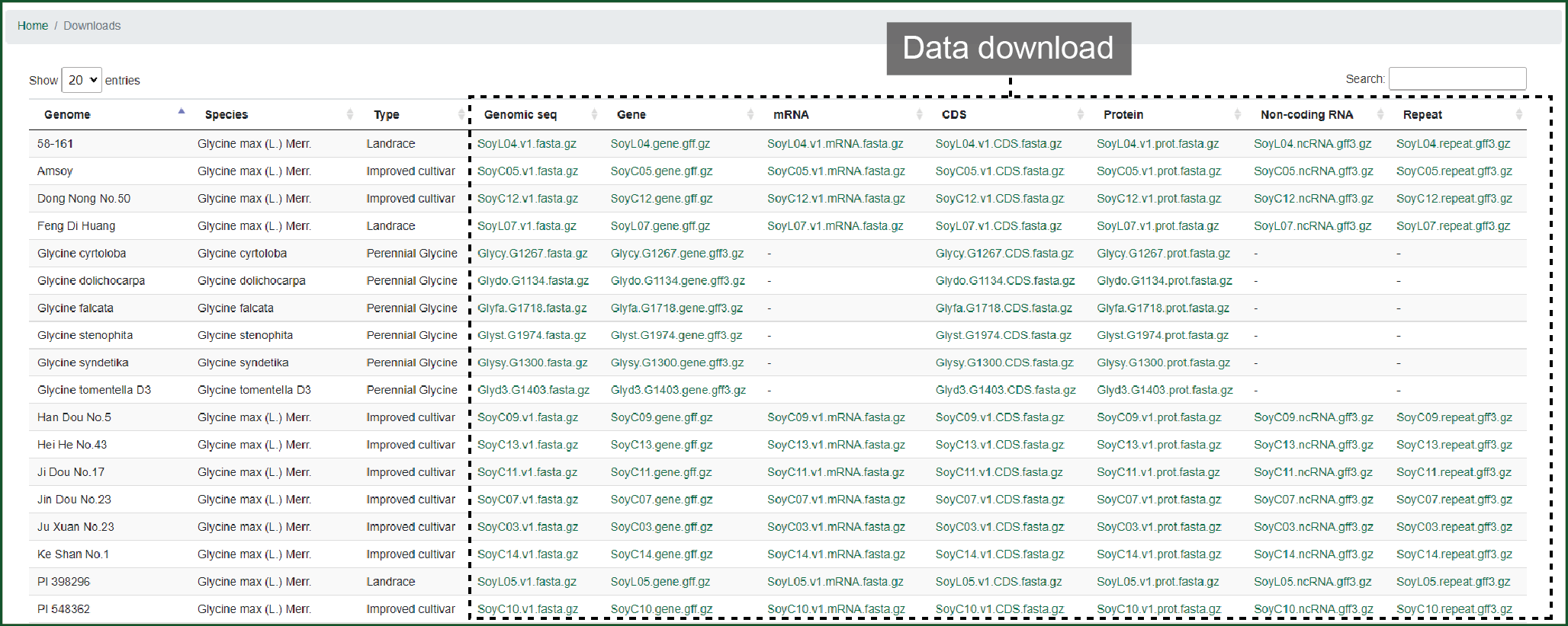
Figure 12 Downloads